Curve Interpretation Part 5: TMA Curves

The interpretation of TMA curves is often difficult because different physical effects produce the same or similar effects on the measurement curves. In such cases, we must either vary the measurement parameters used for the TMA measurement (measurement mode, force program, temperature program) or obtain more information by using other thermal analysis methods. In this article, we discuss a number of practical approaches.

Introduction

Depending on the method and mode used for the actual measurement, it is not always possible to uniquely assign effects on a TMA curve to particular physical processes. For example, a steplike change to shorter length in a measurement performed in compression can indicate a glass transition, melting or a solid-solid transition. In such cases, additional measurements are needed to interpret the measured TMA curve. Some possibilities are:

• to vary the force program using different static forces (positive or negative) or oscillating forces (DLTMA);
  
• to vary the temperature program using heating-cooling-heating cycles or by changing the heating rate; 
  
• to use a different measurement mode (e.g. expansion instead of compression);
  
• to use a different thermal analysis technique such as DSC, TGA (-EGA) or DMA.
  

In this article, we will show how these possibilities can lead to a better understanding of the processes occurring in a material.

Influence of the Force Program

In a TMA measurement, the force program used has a decisive influence on the shape of the measurement curve. For example, if an amorphous material is measured using a small force, the glass transition appears as an increase in the slope of the TMA curve (the TMA curve becomes steeper).

If the same sample is measured using a large force, the glass transition is observed as a step in the TMA curve (the thickness of the sample decreases). The TMA provides forces ranging from –0.1 N to +1 N. In addition force programs can be used in which the applied force is not constant but varies as a sine wave or square wave function.

Example 1

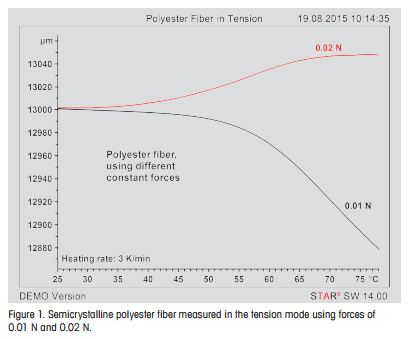
Figure 1 shows the shrinkage and expansion behavior of a polyester fiber. The measurement of shrinkage usually requires the use of low forces. The black curve was recorded using a constant force of 0.01 N. We see that the sample shrinks (the sample length decreases).

The red curve was measured using a force of 0.02 N. Here we see that the fiber stretches after the glass transition. The shrinkage force of the material (the force at which the sample neither shrinks nor stretches) therefore lies between 0.01 N and 0.02 N for the sample measured here.

Shrinkage is typical for semicrystalline stretched fibers: as a result of the production process, the crystals are all oriented in the same direction. This orientation is lost after the glass transition and the fibers shrink in the direction of tension (and become thicker). Comparison of materials in this way allows conclusions to be drawn about differences in production and about the materials themselves.

Example 2: DLTMA

In Dynamic Load TMA or DLTMA, the force acting on the sample varies. We can use either a sine wave or a square wave force program. In the square wave force program, the applied force changes periodically from a smaller to a larger value. The values of the two forces and the period (the default value is 12 s) have to be specified in the method.

In the sine wave force program, the applied force varies as a sine function between two forces that also have to be specified in the method. In this case, the period can also be freely chosen. Figure 2 shows the result of a DLTMA measurement of a thin 0.5-mm polyethylene terephthalate (PET) disk. For comparison, the curve in the upper diagram shows the TMA measurement of the same material performed in compression using a constant force.

The TMA curve shows three clear steps in which the thickness of the sample decreases as the measurement probe penetrates more and more into the sample.

The measurement does not however allow us to unambiguously assign the three effects - they could be due to a glass transition, melting, crystallization, shrinkage, decomposition, or other effects.

The DLTMA experiment provides us with the information we need to interpret the TMA measurement curve [1]. Up until about 70 °C, the change in force has no effect and the material is hard. At about 70 °C, the sample softens and the displacement amplitude increases. At the same time, the material expands and there is a sudden change in the coefficient of thermal expansion (CTE).

This behavior is typical for a glass transition. The amplitude then decreases, the material becomes harder and shrinks. The behavior is characteristic for cold crystallization. After this transition, the displacement amplitude is almost zero and the material is now hard again but crystalline and no longer amorphous. Now that we have assigned the first two steps, the final step can only be due to the melting of crystallites formed.

Example 3: DLTMA with positive and negative forces

DLTMA measurements are usually performed using positive forces. Certain applications however need alternating positive and negative forces. An example of this is shown in Figure 3, which displays measurement curves of an initially liquid adhesive. The adhesive was contained in a 40-µL aluminum crucible to prevent it flowing. The measurement was performed using a flat measurement probe (surface area 1 mm2 ) at a constant temperature of 10 °C.

The force program is shown in the upper right corner of the diagram. The DLTMA curve (black) initially shows very large deflections. As long as the sample is liquid, the negative force lifts the probe completely out of the liquid.

Conclusions

Depending on the method and mode used for the actual measurement, it is not always possible to definitely assign effects on a TMA curve to particular physical processes. In such cases, measurements performed under other conditions can lead to a better understanding of the processes that occur in the material.

The possibilities include measurements using different force programs (static force, DLTMA, DLTMA with different frequencies), measurements using a different measurement mode (for example expansion instead of penetration) or measurements using a different temperature program (heating-cooling-heating, variation of the heating rate). In many cases, the use of other thermal analysis techniques (DSC, TGA-EGA or DMA) can also provide important information to help you interpret TMA curves.

_{Curve Interpretation Part 5: TMA Curves | Thermal Analysis Application No. UC 421 | Application published in METTLER TOLEDO Thermal Analysis UserCom 42}