Evaluation and Interpretation of Peak Temperatures of DSC Curves. Part 1: Basic Principles

Introduction 

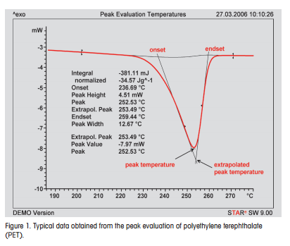
The determination of different characteristic values of peaks is one of the most frequent evaluations performed in DSC. Some of these quantities are shown in the curve in Figure 1. For example, the integral is determined by integrating the area under the peak and yields the transition enthalpy, Δh. Equally important are the onset temperature, T_on, (especially with the melting of pure materials) and the temperature of the peak maximum (the peak temperature, T_m) because they are directly related to characteristic values of the material under investigation. For example, with pure substances, the onset temperature is the melting temperature.

However, if peaks are broad, the onset temperature cannot be precisely determined and it loses its physical meaning. The peak temperature is then used to define the melting temperature.

In the case of polymers, the peak temperature, T_m, is a measure of the average melting temperature of the crystallites. With second order phase transitions, T_m is the characteristic temperature of the transition, and with mixtures, the peak maximum defines the liquidus curve in the phase diagram.

While the values measured for Δh and T_on are largely independent of the heating rate, B, and sample mass, m, the peak temperature is very dependent on these two parameters. Larger sample masses and higher heating rates shift the peak maximum to higher temperatures. Furthermore, in contrast to Ton, one notices that the peak temperature can be quite different (Figure 2) depending on whether the curve is displayed as a function of the sample temperature or the program temperature (in the STAR^e software terminology, the reference temperature). This question then arises as to what is the “true peak temperature” and what does it mean, or at least, what is the best approach for evaluating the peak. These topics will be discussed in particular in connection with melting processes in this two-part article series. 

Part 1 here deals with the origin of a DSC melting peak and derives the properties of an ideal melting peak. In Part 2, these ideas will be applied and illustrated with the aid of practical examples.

The Ideal Melting Peak 

The following sections discuss the influence of the sample and measurement conditions on peak temperature using a very simple model. First, the model refers to a thin sample of good thermal conductivity in which temperature gradients do not occur. The heat capacity of the sample before and after the transition is the same. The thermal behavior of the sample and reference sides of the measuring system is perfectly symmetrical. Finally, the response of the instrument to a sudden change in heat flow is a pure exponential function. 

Conclusions

During a melting peak, differences occur between the program temperature and the measured and true sample temperatures as a result of the corresponding heat transfer processes. The resulting temperature gradients give rise to the peaks measured in the heat flow curve.

The peak temperature, T_m, depends on the measurement conditions (heating rate, sample mass, heat transfer) and is not a direct measure for a material property. If you want to compare this quantity meaningfully for different samples, the measurements must be performed at the same heating rate using samples of similar mass contained in the same type of crucible. The peak temperature extrapolated to a mass and heating rate of zero is obtained using the Illers diagram. This quantity is independent of the experimental conditions and corresponds to the equilibrium melting temperature of the crystallites present. The temperatures of the peak evaluation (onset and peak temperatures) differ depending on whether the evaluation is performed as a function of the program temperature (STAR^e terminology: reference temperature) or the sample temperature. The evaluation of the peak as a function of the sample temperature yields results that are closer to the true sample temperature.

In the STAR^e software, the DSC curves can be displayed using the program temperature (reference temperature) or the sample temperature. The evaluation mode can be set in the results mode. This means that the evaluation of a measurement curve displayed as a function of the reference temperature can also provide the corresponding sample temperatures.

In Part 2 of this series, a number of real measurement curves will be discussed.

_{Evaluation and Interpretation of Peak Temperatures of DSC curves. Part 1: Basic Principles | Thermal Analysis Application No. UC 232 | Application published in METTLER TOLEDO Thermal Analysis UserCom 23}