Model Free Kinetics
Introduction
The kinetics of chemical reactions can be easily determined from DSC or TGA measurements. The METTLER TOLEDO STARe software offers three different software options: the classical nth order kinetics and two so-called model-free methods.
The nth order kinetics approach assumes that the activation energy is constant throughout the entire reaction. The reaction rate, dα/dt, is given by the equation where α is the conversion, K0 is the pre-exponential factor, Ea the activation energy, R the gas constant, T the temperature and n the order of the reaction. An nth order reaction is therefore completely described by the parameters n, Ea and K0. This model is, however, at best only suitable for simple reactions. In more complex reactions in which several reaction steps proceed in parallel, or in which the reaction is not completely chemically controlled, nth order kinetics fails. In such cases, model free kinetics is an excellent alternative to describe the reaction kinetics
This study shows how model free kinetics can be used to evaluate DSC and TGA measurements and make predictions about the isothermal behavior of reactions (i.e. determine conversion as a function of time at a certain temperature, or the time needed at a given temperature to reach a certain conversion).
Basic Principles of Model Free Kinetics
Model free kinetics assumes that the activation energy does not remain constant during a reaction but changes. Furthermore, it assumes that the activation energy at a particular conversion is independent of the temperature program (the “iso-conversion principle”).
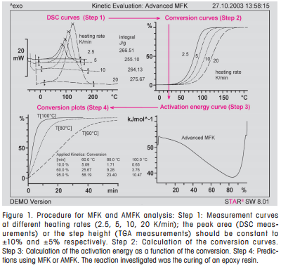
In the STAResoftware, two different versions of model free kinetics have been implemented as software evaluation options: the standard model free kinetics (MFK, Model Free Kinetics) and the advanced model free kinetics (AMFK, Advanced Model Free Kinetics). The difference between these two approaches is to be found in the numerical algorithms that are used for the evaluation. Furthermore, with standard MFK, only dynamic heating curves can be evaluated. With AMFK, however, curves can be evaluated that have been measured with any temperature program, including isothermal measurements.
Experimental Details
As “raw data”, model free kinetics requires at least three DSC or TGA curves measured with different temperature programs. First of all, it is always best to make a trial run in order to first get a general impression of the “reaction profile”, that is, the temperature range, reaction enthalpy and mass loss. Relatively slow heating rates (e.g. 5 K/min) should be used for materials that release large amounts of energy during the reaction (e.g. explosives). For safety reasons it is advisable to use high-pressure crucibles and low sample masses (< 5 mg). With other materials, heating rates of 10 or 20 K/min can be used for the trial run.
For MFK, a minimum of three experiments must be performed at different heating rates. Four or five measurements are however recommended to improve the reliability of the calculated predictions. The heating rates used should increase in large steps such as 1, 2, 5, 10, and 20 K/min. The use of smaller steps, for example 5, 6, 7, 8, 9 K/min, reduces the accuracy of the results. At increasing heating rates, chemical reactions take place at higher temperatures. Accordingly, the temperature range must match the heating rate. Particularly when high heating rates are used, for example with curing reactions, (undesired) decomposition reactions frequently occur toward the end of the reaction under investigation. In such cases, lower heating rates should be used.
As mentioned above, isothermal temperature programs can be used for AMFK. As a rule, the temperatures used are below the peak temperature. The reason for this is that above the peak temperature the reaction is very rapid, which makes correct evaluation of the curves difficult. A fundamental problem with isothermal DSC experiments is that at the beginning of the experiment the initial deflection and chemical reaction overlap. In this case, the DSC curve of a second run of the same sample (which should then no longer show any reaction) measured under otherwise identical conditions can be used as the baseline. Just as with MFK, at least three measurements must be made with different temperature programs for AMFK. Four measurements are however also recommended for AMFK; dynamic measurements can be combined with isothermal measurements. With AMFK, the rate at which the measurement values are recorded should be set to the maximum value of 10 measurement values per second.
As far as sample preparation is concerned, it is important to make sure that all the samples are prepared in exactly the same way. In particular, the sample mass should be about the same for all samples. And obviously the crucibles used must not react with the sample. Furthermore, it should be noted that the size of the hole in the crucible lid could influence reactions in which gases are liberated.
Evaluations
The typical revaluation procedure used for MFK and AMFK is illustrated in the example shown in Figure 1 (for DSC measurements).
Conclusions
Model free kinetics allows even complex chemical reactions to be analyzed using just a few DSC or TGA measurements and without making any assumptions about a particular reaction model. The STARe software has implemented two equivalent procedures (MFK and AMFK software options). From the mathematical point of view, the two approaches differ in the numerical algorithms used.
The main difference for the user is that MFK can only evaluate heating curves, but AMFK can in addition evaluate isothermal or combinations of isothermal and dynamic measurements. Both procedures usually yield somewhat different activation energies. However, with regard to predictions, MFK and AMFK give very similar results.
Model Free Kinetics | Thermal Analysis Application No. UC 212 | Application published in METTLER TOLEDO Thermal Analysis UserCom 21

