Evaluation and Interpretation of Peak Temperatures of DSC Curves. Part 2: Examples

Introduction 

In Part 1 of this series [1], the basic principles concerning the formation of peaks in DSC are discussed. It is shown that the peak temperature depends on the heating rate, the sample mass and the thermal contact between the sample and sensor (and thus on the crucible and the purge gas used). Besides this, different peak temperatures are obtained depending on whether the evaluation is performed using the sample temperature or the program temperature (in the STARe terminology the reference temperature). Finally it was shown that in the melting process the peak temperature follows the equation

Tm=Tm,0 + √(2R ΔH)√mβ  (1)

Here, T_m is the peak temperature, T_m,₀ is the peak temperature extrapolated to a heating rate and mass of zero, R is the relevant thermal resistance, Δh is the specific enthalpy of fusion, m is the sample mass and b is the heating rate. If the peak temperature is plotted against the square root of the product of the sample mass and heating rate, a straight line is obtained whose slope depends on the specific enthalpy of fusion and the thermal resistance. The ordinate intercept of the temperature axis is Tm,0. We call a diagram such as this an Illers diagram because Illers first derived equation (1) and experimentally verified its validity for polymer melts [2].

The extrapolated peak temperature, T_m,₀, corresponds to the equilibrium melting temperature of the crystallites melting at the peak maximum.

Based on the discussions in reference [1], approaches for evaluating peak temperatures are discussed using practical examples. This deals mainly with melting processes but also refers to peak evaluation in other processes.

Melting of Pure Materials

The melting behavior of indium is used as an example to show the dependence of peak temperature on the experimental conditions. The melting temperature corresponds to the onset temperature of 156.6 °C. Four samples of different mass (0.053 mg, 0.846 mg, 3.425 mg and 6.301 mg) were measured at heating rates between 1 K/min and 20 K/min. The sample was enclosed in a light aluminum crucible (20 µL; 21.9 mg aluminum). The program temperature, T_m,_p, and the sample temperature, T_m,_s, at the peak maximum were determined. Figure 1 shows the peak temperatures (black circles) in the Illers diagram. The results show that all the measurement points behave according to equation (1). 

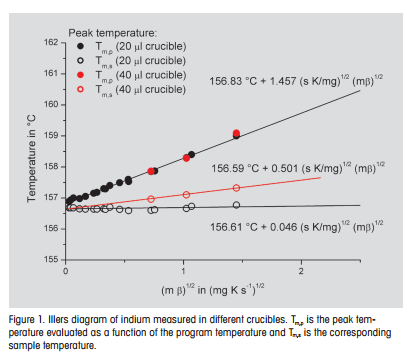
The evaluation using sample temperature gives a much more gradual slope than that using the program temperature. The reason for this is the different thermal resistance relevant for the particular measurement. In the evaluation using the program temperature, it is the resistance between the sample and the furnace, R_f . In the case of the sample temperature, it is the resistance between the sample and the sensor, R_s.

To demonstrate the influence of the crucible, a sample (6.301 mg) was measured in a 40-µL crucible (49.7 mg aluminum) at 5, 10 and 20 K/min. The corresponding peak temperatures are shown in Figure 1 as red circles. The sample temperature curves differ significantly depending on the type of crucible. The larger slope obtained with the 40-µL crucible can be explained by the somewhat larger thermal resistance between sample and sensor. In the evaluation as a function of the program temperature, the difference between these crucibles can be neglected because the thermal resistance between the sample and the furnace is many times larger.

The intercepts of the regression curves in Figure 1 yield the peak temperature extrapolated to a heating rate of zero. This should be the true melting temperature. As expected, it is 156.6 °C for both crucibles. The value is a little higher (156.8 °C) in the evaluation using the program temperature because the sample temperature was calibrated and not the program temperature. The temperature difference, ΔT, of 0.2 K corresponds to the difference between the sample temperature, T_s, and the program temperature, T_p [1].

These measurements show that the melting temperature can be determined from the peak temperature by extrapolating to a heating rate of zero in the Illers diagram. The evaluation should be performed using the sample temperature.

The Melting Peak in the Case of Metastable Crystallites (Polymers)

In contrast to the melting behavior of pure metals, the melting peaks of semicrystalline polymers are often very broad. For this reason, an evaluation of the onset temperature does not provide representative and comparable values.

Conclusions

The peak temperature is an important quantity in the evaluation of thermal events in DSC. It is, however, influenced by the actual experimental conditions. 

To interpret and determine characteristic data, one has to know which thermal event is responsible for the peak. The following rules are helpful for this:

• Determine the mass of the sample before and after the measurement.
  
• Measure the sample on heating, cooling and heating a second time.
  
• Possibly repeat the measurement in sealed (or pierced lid) crucibles.
  
• Repeat the measurement at a different heating rate. 
  

If materials are to be compared using DSC measurements, the measurements must be performed at the same heating rate using a similar sample mass. Especially with polymers and polymorphic materials, melting behavior depends on thermal history such as cooling rate and storage conditions. These parameters must therefore also be taken into account in any comparison.

In general, peak temperature determination should be performed using the sample temperature. If the equilibrium temperatures in melting processes are required, the peak temperature must be measured using at least four different heating rates and the evaluation should be performed using the Illers diagram with extrapolation to a heating rate of zero. Information is then obtained about possible recrystallization processes during the measurement.

If a pure substance is available, the slope of the melting peak can be used to correct the measured peak temperature of melting processes of impure samples. Finally, the peak temperature can be determined with better accuracy if small sample masses are used.

_{Evaluation and Interpretation of Peak Temperatures of DSC Curves. Part 2: Examples | Thermal Analysis Application No. UC 242 | Application published in METTLER TOLEDO Thermal Analysis UserCom 24}